Reveal multiple level of biological heterogeneities in Mouse Hypothalamus by MERFISH-seq¶

In this tutorial, we will showcae the STEP for revealing multiple levels of biological heterogeneities in the Mouse Hypothalamus by MERFISH-seq. STEP has been designed to shed light on different aspects of cellular complexity: 1. Cell State Level Heterogeneity: STEP can capture unique cellular states based on genetic expressions in the mouse hypothalamus. 2. Spatial Domain Level Heterogeneity: STEP facilitates understanding of spatial patterns and relationships among cells by smoothing the cell state embeddings. 3. End-to-End (e2e) Mode for Direct Spatial Domain Identification: A streamlined process to directly identify and analyze spatial heterogeneity.

The aim of this tutorial is to guide users through the process of utilizing and understanding the capabilities of STEP, enabling users to dive deep into the biological intricacies of the mouse hypothalamus.

[1]:

import os
import anndata as ad
import scanpy as sc
import numpy as np
import seaborn as sns
import matplotlib.pyplot as plt
import pandas as pd

from step import scModel, stModel
sc.settings.figdir = './results/MERFISH'
sc.set_figure_params(dpi_save=300, figsize=(6, 4.5))

st_file = './data/merfish_animal1.h5ad'

/projects/82505004-e7a0-445f-ab3c-80d03c91438f/.cache/pypoetry/virtualenvs/step-Ajq_Bw_i-py3.10/lib/python3.10/site-packages/tqdm/auto.py:21: TqdmWarning: IProgress not found. Please update jupyter and ipywidgets. See https://ipywidgets.readthedocs.io/en/stable/user_install.html
  from .autonotebook import tqdm as notebook_tqdm

Cell state level heterogeneity¶

For the identification of cell state level hetorogeneity single-cell resolution data, we use step.scModel which will focus on the modeling of transcipts and elimination of the potential batch-effects (not presented in this data), ignoring the spatial context even though the data is spatially resovled.

Setup STEP object¶

Due to the limitation of the MERFISH technique, there’re only 161 genes across sections. Subsequently, we will use all these genes by setting the paramter n_top_genes=None and set the parameter n_modules=20 to model the fewer gene modules.

[2]:

stepc = scModel(
    file_path=st_file,
    n_top_genes=None,
    layer_key=None,
    batch_key='Bregma',
    class_key='Cell_class',
    module_dim=30,
    hidden_dim=64,
    n_modules=20,
    decoder_type='zinb',
    n_dec_hid_layers=1,
)

Using all genes
Using given geneset
Adding count data to layer 'counts'
================Dataset Info================
Batch key: Bregma
Class key: Cell_class
Number of Batches: 5
Number of Classes: 15
Gene Expr: (28316, 161)
Batch Label: (28316,)
============================================

[3]:

stepc.adata.obs.head()

[3]:

	Animal_ID	Animal_sex	Behavior	Bregma	Centroid_X	Centroid_Y	Cell_class	Neuron_cluster_ID	in_tissue	n_genes
Cell_ID
6c59b1ec-95df-4f25-882a-ac94d99b87d8	1	Female	Naive	-0.04	-3033.401378	2825.155877	Endothelial 3	NaN	True	29
aa7ce410-c485-42c9-9c29-bc1d90a46e00	1	Female	Naive	-0.04	-3027.328655	2955.936449	Inhibitory	I-5	True	61
8426329e-077b-4385-bd94-c9fdaeb89bd1	1	Female	Naive	-0.04	-3020.512953	2961.696710	Inhibitory	I-5	True	54
a7e4e0de-8baa-4136-8cac-fa9bc759e7e8	1	Female	Naive	-0.04	-3017.397490	2995.915801	Inhibitory	I-5	True	86
c55468d5-1b2c-4477-b4ad-3653f5bbda35	1	Female	Naive	-0.04	-3005.478613	2877.528929	Endothelial 1	NaN	True	40

[4]:

stepc.run(epochs=400,
          batch_size=2048,
          split_rate=0.2,
          tune_epochs=100,
          beta1=0.1,
          beta2=0.01,
         )

================Dataset Info================
Batch key: Bregma
Class key: Cell_class
Number of Batches: 5
Number of Classes: 15
Gene Expr: (28316, 161)
Batch Label: (28316,)
============================================
Performing category random split
Training size for -0.24: 4434
Training size for -0.19: 4641
Training size for -0.14: 4740
Training size for -0.09: 4445
Training size for -0.04: 4390
train size: 22650
valid size: 5666
Current Mode: multi_batches: ['gene_expr', 'batch_label']
Current Mode: multi_batches: ['gene_expr', 'batch_label']
100%|██████████| 400/400 [05:15<00:00,  1.27epoch/s, kl_loss=2.391, recon_loss=160.094, val_kl_loss=2.473/2.288, val_recon_loss=154.405/153.951]
Current Mode: multi_batches: ['gene_expr', 'batch_label']
Current Mode: multi_batches: ['gene_expr', 'batch_label']
Current Mode: multi_batches_with_ct: ['gene_expr', 'class_label', 'batch_label']
================Dataset Info================
Batch key: Bregma
Class key: Cell_class
Number of Batches: 5
Number of Classes: 15
Gene Expr: (28316, 161)
Class Label: (28316,)
Batch Label: (28316,)
============================================
Performing category random split
Training size for Astrocyte: 2724
Training size for Endothelial 1: 1184
Training size for Endothelial 2: 115
Training size for Endothelial 3: 439
Training size for Ependymal: 1029
Training size for Excitatory: 4629
Training size for Inhibitory: 9895
Training size for Microglia: 475
Training size for OD Immature 1: 809
Training size for OD Immature 2: 25
Training size for OD Mature 1: 190
Training size for OD Mature 2: 922
Training size for OD Mature 3: 11
Training size for OD Mature 4: 37
Training size for Pericytes: 163
train size: 22647
valid size: 5669
Current Mode: multi_batches_with_ct: ['gene_expr', 'class_label', 'batch_label']
Current Mode: multi_batches_with_ct: ['gene_expr', 'class_label', 'batch_label']
 32%|███▏      | 32/100 [00:31<01:04,  1.05epoch/s, cl_loss=0.036, kl_loss=0.009, val_cl_loss=0.317/0.233, val_kl_loss=0.010/0.010]Early Stopping triggered
 32%|███▏      | 32/100 [00:31<01:06,  1.03epoch/s, cl_loss=0.036, kl_loss=0.009, val_cl_loss=0.317/0.233, val_kl_loss=0.010/0.010]
Current Mode: multi_batches: ['gene_expr', 'batch_label']

EarlyStopping counter: 20 out of 20
EarlyStopping counter: 2 out of 1

Current Mode: multi_batches_with_ct: ['gene_expr', 'class_label', 'batch_label']
Current Mode: multi_batches: ['gene_expr', 'batch_label']
Current Mode: multi_batches: ['gene_expr', 'batch_label']
Current Mode: multi_batches: ['gene_expr', 'batch_label']

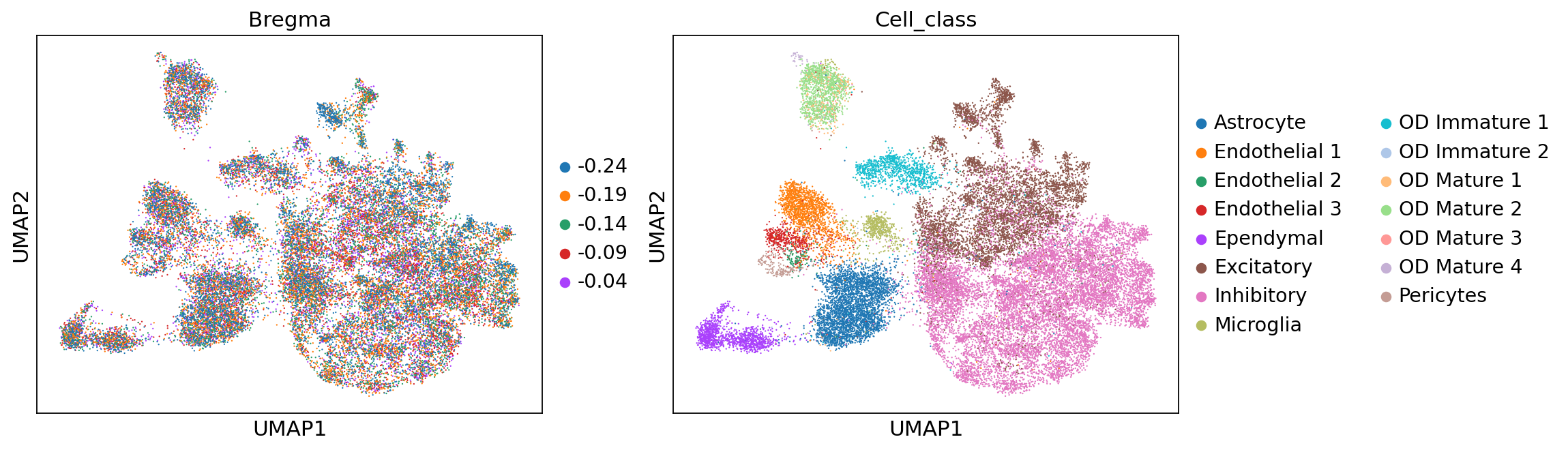
[11]:

adata = stepc.adata

sc.pp.neighbors(adata, use_rep='X_rep')
sc.tl.umap(adata)
sc.pl.umap(adata, color=['Bregma', 'Cell_class'])

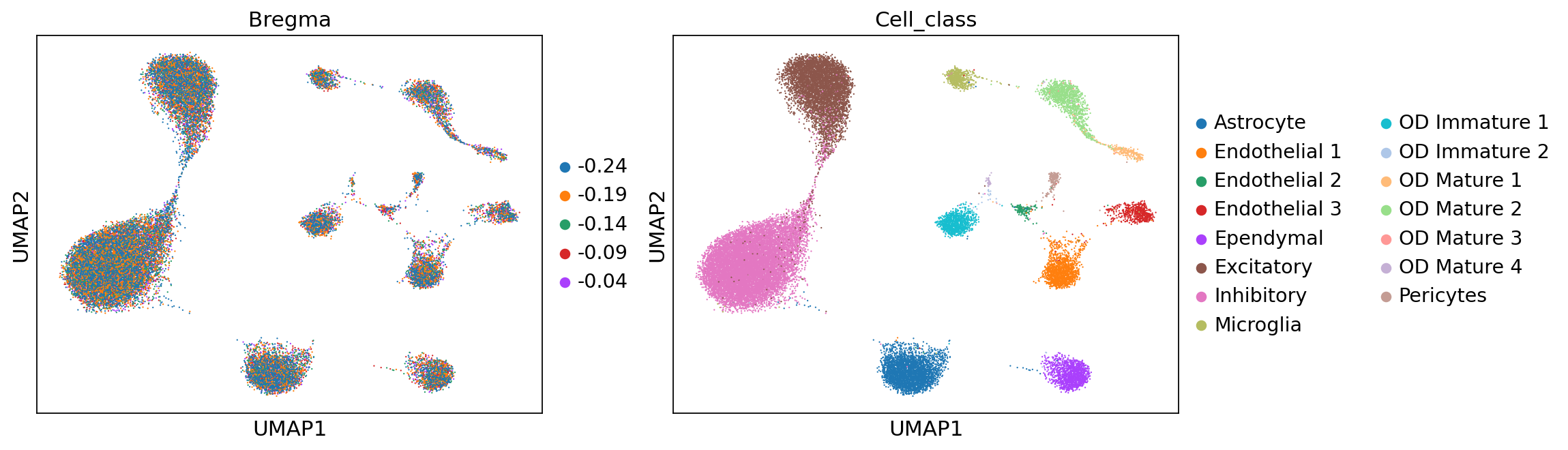
[12]:

sc.pp.neighbors(adata, use_rep='X_anchord')
sc.tl.umap(adata)
sc.pl.umap(adata, color=['Bregma', 'Cell_class'])

[15]:

from scib_metrics.benchmark import Benchmarker, BioConservation

biocons = BioConservation(nmi_ari_cluster_labels_leiden=True, nmi_ari_cluster_labels_kmeans=False)
# batcons = BatchCorrection(pcr_comparison=False)
bm = Benchmarker(
    adata,
    batch_key="Bregma",
    label_key="Cell_class",
    embedding_obsm_keys=["X_rep", "X_anchord", "X_pca_corrected", "X_pca"],
    bio_conservation_metrics=biocons,
    # batch_correction_metrics=batcons,
    n_jobs=-1,
)
bm.benchmark()
bm.plot_results_table(min_max_scale=False)

Computing neighbors: 100%|██████████| 2/2 [00:09<00:00,  4.70s/it]
Embeddings:   0%|          | 0/2 [00:00<?, ?it/s]
Metrics:   0%|          | 0/10 [00:00<?, ?it/s]
Metrics:   0%|          | 0/10 [00:00<?, ?it/s, Bio conservation: isolated_labels]WARNING:jax._src.xla_bridge:An NVIDIA GPU may be present on this machine, but a CUDA-enabled jaxlib is not installed. Falling back to cpu.

Metrics:  10%|█         | 1/10 [00:02<00:20,  2.30s/it, Bio conservation: isolated_labels]
Metrics:  10%|█         | 1/10 [00:02<00:20,  2.30s/it, Bio conservation: nmi_ari_cluster_labels_leiden]
Metrics:  20%|██        | 2/10 [00:10<00:46,  5.78s/it, Bio conservation: nmi_ari_cluster_labels_leiden]
Metrics:  20%|██        | 2/10 [00:10<00:46,  5.78s/it, Bio conservation: silhouette_label]
Metrics:  30%|███       | 3/10 [00:12<00:27,  3.94s/it, Bio conservation: silhouette_label]
Metrics:  30%|███       | 3/10 [00:12<00:27,  3.94s/it, Bio conservation: clisi_knn]
Metrics:  40%|████      | 4/10 [00:13<00:16,  2.69s/it, Bio conservation: clisi_knn]
Metrics:  40%|████      | 4/10 [00:13<00:16,  2.69s/it, Batch correction: silhouette_batch]
Metrics:  50%|█████     | 5/10 [00:19<00:19,  3.93s/it, Batch correction: silhouette_batch]
Metrics:  50%|█████     | 5/10 [00:19<00:19,  3.93s/it, Batch correction: ilisi_knn]
Metrics:  60%|██████    | 6/10 [00:19<00:10,  2.67s/it, Batch correction: ilisi_knn]
Metrics:  60%|██████    | 6/10 [00:19<00:10,  2.67s/it, Batch correction: kbet_per_label]
Metrics:  70%|███████   | 7/10 [00:35<00:21,  7.01s/it, Batch correction: kbet_per_label]
Metrics:  70%|███████   | 7/10 [00:35<00:21,  7.01s/it, Batch correction: graph_connectivity]
Metrics:  80%|████████  | 8/10 [00:35<00:14,  7.01s/it, Batch correction: pcr_comparison]
Embeddings:  50%|█████     | 1/2 [00:36<00:36, 36.03s/it]atch correction: pcr_comparison]
Metrics:   0%|          | 0/10 [00:00<?, ?it/s]

Metrics:   0%|          | 0/10 [00:00<?, ?it/s, Bio conservation: isolated_labels]
Metrics:  10%|█         | 1/10 [00:01<00:16,  1.83s/it, Bio conservation: isolated_labels]
Metrics:  10%|█         | 1/10 [00:01<00:16,  1.83s/it, Bio conservation: nmi_ari_cluster_labels_leiden]
Metrics:  20%|██        | 2/10 [00:11<00:50,  6.26s/it, Bio conservation: nmi_ari_cluster_labels_leiden]
Metrics:  20%|██        | 2/10 [00:11<00:50,  6.26s/it, Bio conservation: silhouette_label]
Metrics:  30%|███       | 3/10 [00:12<00:29,  4.17s/it, Bio conservation: silhouette_label]
Metrics:  30%|███       | 3/10 [00:12<00:29,  4.17s/it, Bio conservation: clisi_knn]
Metrics:  40%|████      | 4/10 [00:13<00:15,  2.60s/it, Bio conservation: clisi_knn]
Metrics:  40%|████      | 4/10 [00:13<00:15,  2.60s/it, Batch correction: silhouette_batch]
Metrics:  50%|█████     | 5/10 [00:13<00:09,  1.83s/it, Batch correction: silhouette_batch]
Metrics:  50%|█████     | 5/10 [00:13<00:09,  1.83s/it, Batch correction: ilisi_knn]
Metrics:  60%|██████    | 6/10 [00:13<00:05,  1.27s/it, Batch correction: ilisi_knn]
Metrics:  60%|██████    | 6/10 [00:13<00:05,  1.27s/it, Batch correction: kbet_per_label]
Metrics:  70%|███████   | 7/10 [00:30<00:18,  6.29s/it, Batch correction: kbet_per_label]
Metrics:  70%|███████   | 7/10 [00:30<00:18,  6.29s/it, Batch correction: graph_connectivity]
Embeddings: 100%|██████████| 2/2 [01:06<00:00, 33.24s/it]atch correction: pcr_comparison]

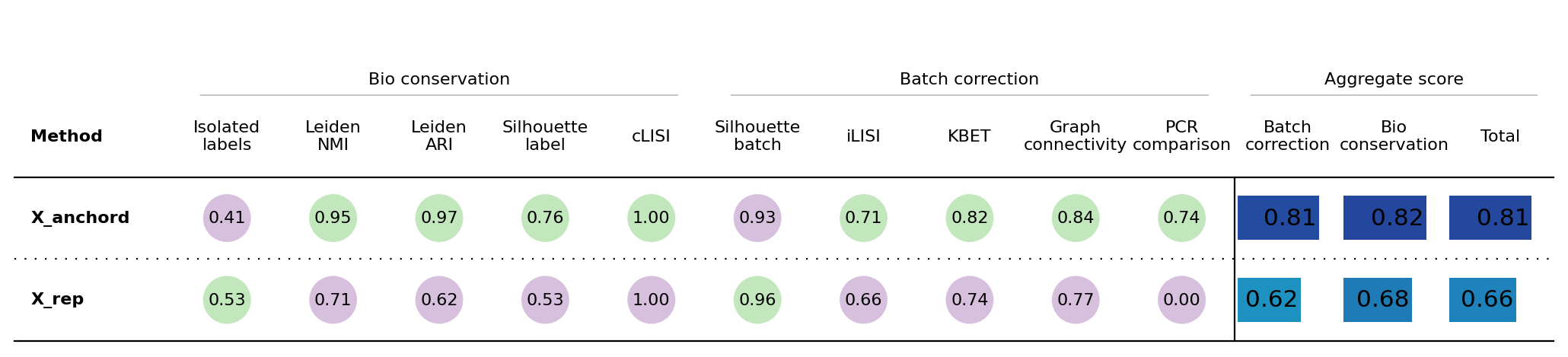
[15]:

<plottable.table.Table at 0x7fdb6c7edd20>

Spatial domain level heterogeneity by spatially smoothing the embedding in cell state level¶

[2]:

model_config = dict(
    n_glayers=4,
    max_neighbors=20,
    variational=True,
)

run_config = dict(
    epochs=400,
    split_rate=0.2,
    n_iterations=800,
    batch_size=1024,
    graph_batch_size=2,
    tune_lr=1e-4,
    beta=1e-4,
    e2e=False,
)

[3]:

stepc = stModel(
    file_path=st_file,
    n_top_genes=None,
    batch_key='Bregma',
    filtered=True,
    layer_key=None,
    log_transformed=True,
    coord_keys=['Centroid_X', 'Centroid_Y'],
    module_dim=30,
    hidden_dim=64,
    n_modules=20,
    decoder_type='zinb',
    edge_clip=None,
    dispersion='gene',
    use_earlystop=True,
    **model_config,
)

Using all genes
Using given geneset
Adding count data to layer 'counts'
Dataset Done
================Dataset Info================
Batch key: Bregma
Class key: None
Number of Batches: 5
Number of Classes: None
Gene Expr: (28316, 161)
Batch Label: (28316,)
============================================

[4]:

stepc.run(**run_config)

Training with 2 stages pattern: 1/2
Performing global random split
100%|██████████| 400/400 [03:48<00:00,  1.75epoch/s, kl_loss=0.880, recon_loss=146.231, val_kl_loss=0.884, val_recon_loss=147.476]
Training graph with multiple batches
Training with 2 stages pattern: 2/2
100%|██████████| 800/800 [07:45<00:00,  1.72epoch/s, kl_loss=0.012, recon_loss=212.722]

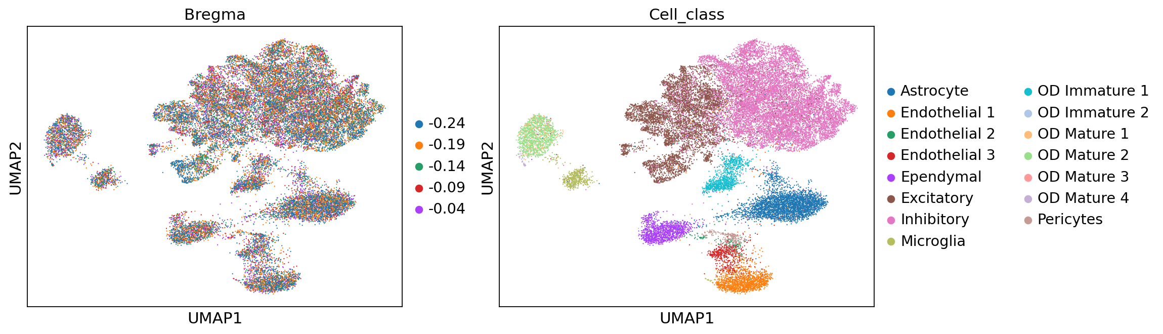
[5]:

adata = stepc.adata

sc.pp.neighbors(adata, use_rep='X_unsmoothed')
sc.tl.umap(adata)
sc.pl.umap(adata, color=['Bregma', 'Cell_class'])

[6]:

stepc.cluster(adata=adata, use_rep='X_smoothed', n_clusters=8)
sc.pp.neighbors(adata, use_rep='X_smoothed')
sc.tl.umap(adata)
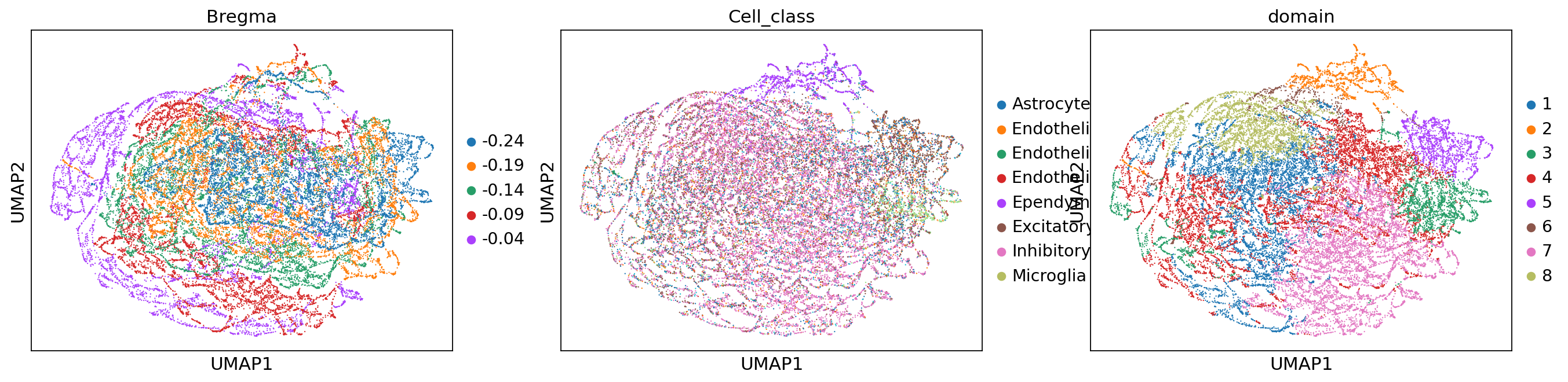
sc.pl.umap(adata, color=['Bregma', 'Cell_class', 'domain'])

[12]:

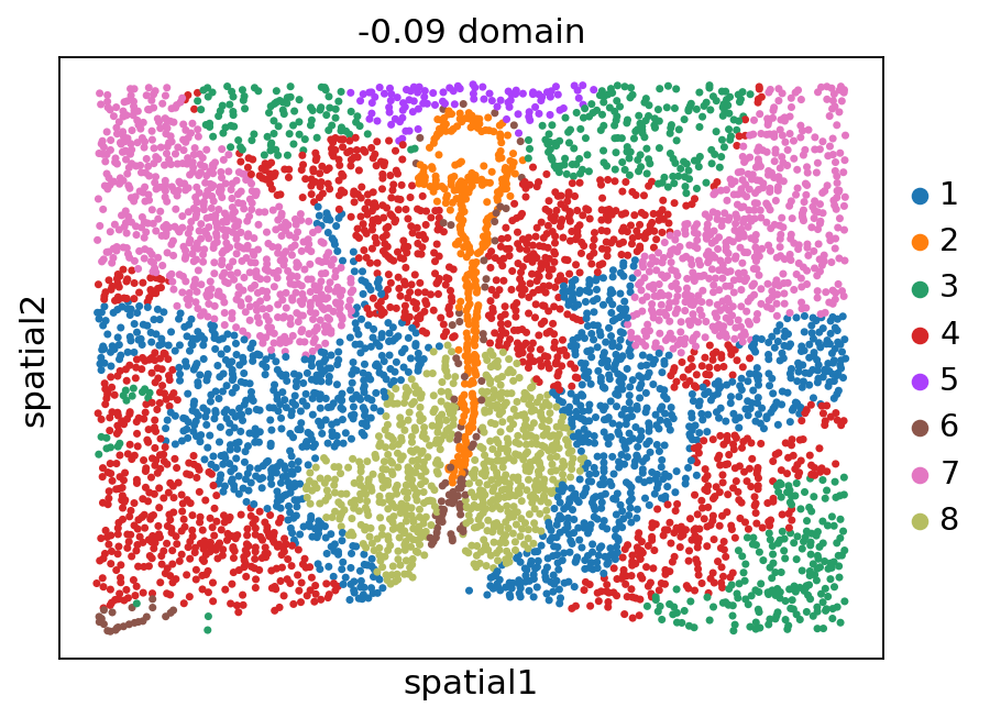
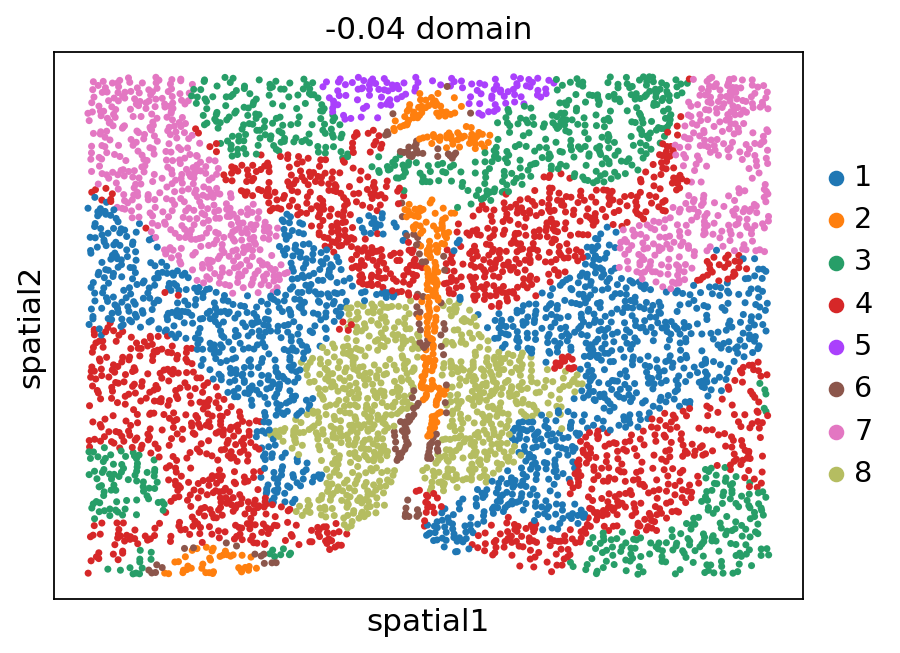
stepc.spatial_plot(color='domain', with_images=False, size=40)

Title not provided, or length does not match the number of batches. Using feature names as title.

E2E mode for direct spatial domain identification¶

Model config & running config¶

First, set e2e=True to enable the e2e mode. In e2e mode, these parameters used in the non e2e mode will be ignored: - epochs - batch_size - split_rate

Instead, a graph sampling strategy will be used to train the model.

[2]:

model_config = dict(
    n_glayers=4,
    max_neighbors=30,
    variational=True,
)

run_config = dict(
    n_iterations=2000,
    graph_batch_size=1,
    beta=1e-2,
    e2e=True,
    contrast=True,
)

Load data and add annotations of zones¶

Note: The annotations of zones is obtained from the tutorial of BASS

[ ]:

adata = sc.read_h5ad(st_file)

for batch in os.listdir('./data/merfish_anno/'):
    anno = pd.read_csv(f'./data/merfish_anno/{batch}', index_col=0)
    batch_id = batch[:-4][6:]
    adata.obs.loc[adata.obs['Bregma'] == float(batch_id), 'annotation'] = anno['x'].values

Set up STEP object¶

[6]:

stepc = stModel(
    adata=adata,
    n_top_genes=None,
    geneset_to_use=adata.var_names,
    batch_key='Bregma',
    filtered=True,
    layer_key=None,
    log_transformed=True,
    coord_keys=['Centroid_X', 'Centroid_Y'],
    module_dim=30,
    hidden_dim=64,
    n_modules=20,
    decoder_type='zinb',
    edge_clip=None,
    **model_config,
)

Adding count data to layer 'counts'
Dataset Done
Modeling with 1 components
{'variational': True, 'input_dim': 161, 'hidden_dim': 64, 'module_dim': 30, 'decoder_input_dim': None, 'n_modules': 20, 'edge_clip': None, 'decoder_type': 'zinb', 'n_glayers': 4}

Generate spatially smoothed embeddings and cluster them to obtain spatial domains¶

[7]:

stepc.run(**run_config)
adata = stepc.adata

Training with e2e pattern
Training graph with multiple batches

100%|██████████| 2000/2000 [04:22<00:00,  7.60step/s, recon_loss=370.799, kl_loss=0.428, contrast_loss=0.011, val_recon_loss=-, val_kl_loss=-, val_contrast_loss=-]

[9]:

stepc.cluster(adata, use_rep='X_smoothed', n_clusters=8,)

Visualization¶

[10]:

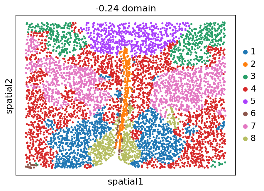
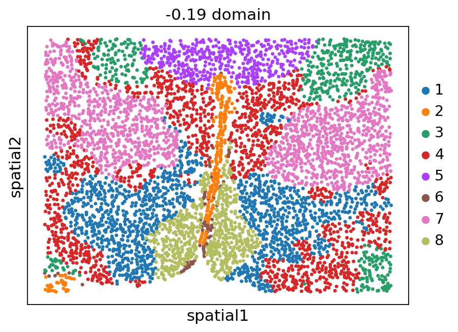
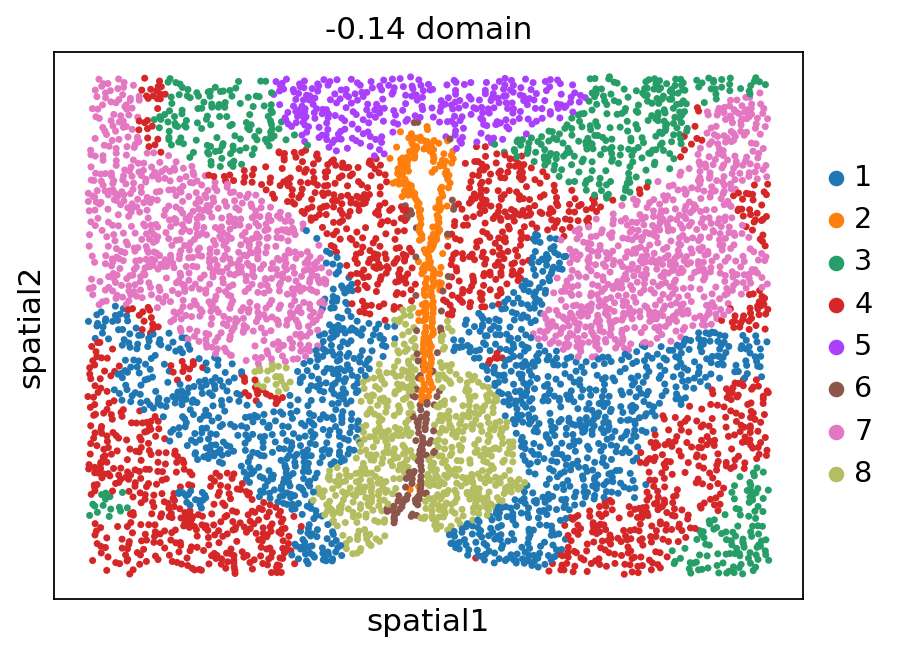
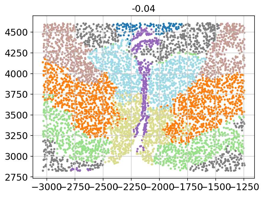
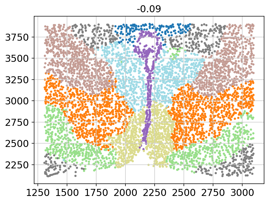
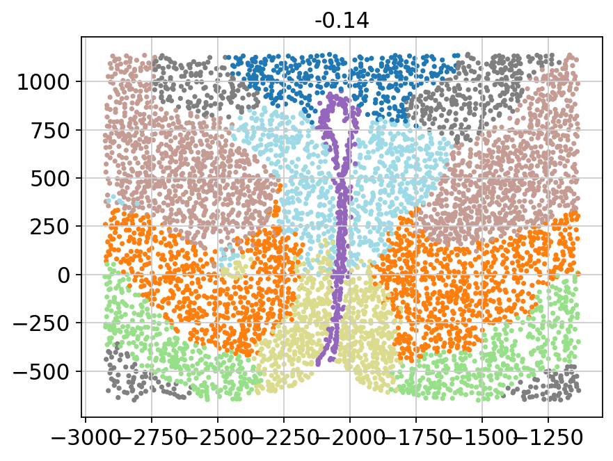
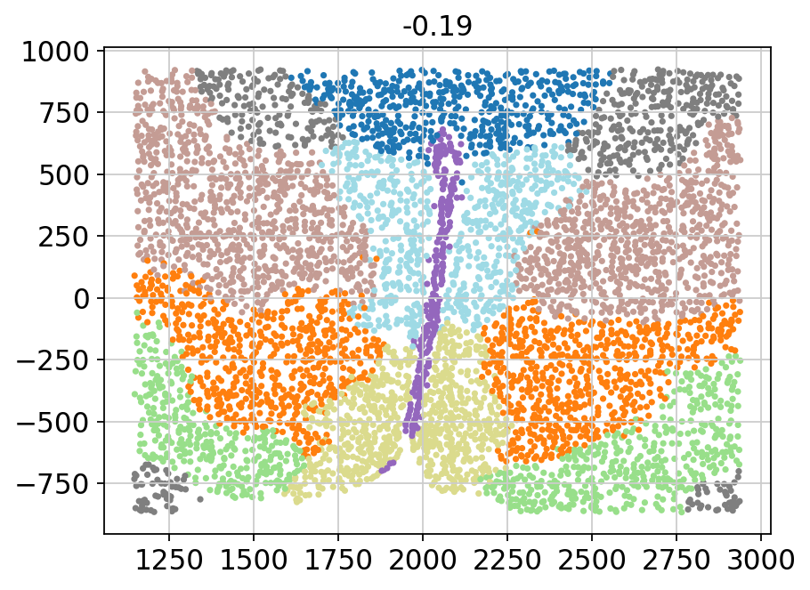
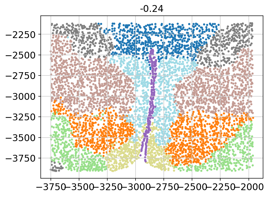
for batch in adata.obs['Bregma'].unique():
    _adata = adata[adata.obs['Bregma'] == batch]
    plt.title(batch)
    plt.scatter(x=_adata.obs['Centroid_X'],
            y=_adata.obs['Centroid_Y'],
            c=_adata.obs['domain'].values.astype(int),
            s=5, cmap='tab20')
    plt.show()

[11]:

adata.obs['annotation'] = adata.obs['annotation'].astype('category')

Metrics for evaluation of the obtained spatial domains compared to the annotations¶

[13]:

from sklearn.metrics import adjusted_rand_score

for batch in adata.obs['Bregma'].unique():
    _adata = adata[adata.obs['Bregma'] == batch]
    ari = adjusted_rand_score(_adata.obs['domain'].astype(int), _adata.obs['annotation'].cat.codes)
    print(f"{batch}: {ari}")

-0.04: 0.5337230222364567
-0.09: 0.6226701393120998
-0.14: 0.49295132575539485
-0.19: 0.6502377274236062
-0.24: 0.6812873877486072